Chapter 8: PMT and PV Functions

In this chapter, you will learn two popularly used financial functions the payment, PMT function, and the present value, PV function.

The PMT Function

Let’s start with the payment, PMT function. To use this function, you must know the interest rate, the number of periods (usually in years or months), and the total value of the loan. This function will produce the total payment which includes both principal and interest.

The Figure below shows an example of the PMT function. This example calculates the monthly personal loan payment for a $5,000 loan amount from the bank for 60 months, with a 4.5% interest rate per year.

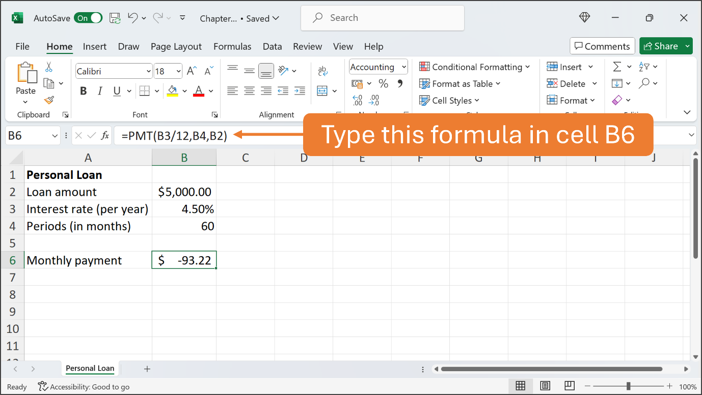
Type the contents in their respective cells. Use the default font and font size. You may format or adjust any column width if necessary. In cell B6, type the formula using the PMT function, =PMT(B3/12,B4,-B2). Press Enter and you get the result.

Let’s look at each required component for the PMT function. The loan amount is given as $5,000.00 in cell B2. You can format cell B2 to Accounting with the dollar symbol, $, and two decimal places (usually it is automatically assigned by Excel). The interest rate is given as 4.50% in cell B3. When you type 4.50% with the % symbol in cell B3, Excel automatically formats the cell from General to Percentage with two decimal places. The period is given as 60 months in cell B4.

The formula in cell B6 is written as =PMT(B3/12,B4,-B2) to get the monthly payment. You can format cell B6 to Accounting with the dollar symbol, $, and two decimal places. The first component in the formula is B3/12 which is the interest rate for the loan. It should be divided by 12 as the interest rate given in cell B3 is yearly, and you need to get the monthly payment, not the yearly payment. The second component in the formula is B4 which is the total number of payments for the loan. The third component in the formula is B2 which is the total loan value. Only three components are required for the PMT function in this example. The other two components are optional.

As a result, Excel returns $ -93.22 in cell B6. It has a negative value as it means payments that should be made from you to the bank. You may get the value in brackets which also means a negative value.

You can rename the worksheet as Personal Loan and later, save the workbook as Chapter8.xlsx.

The PV Function

Now, let’s learn the present value, the PV function. Insert a new worksheet in the same workbook, and rename it Invest Today.

The following Figure shows an example of the PV function. If you expect to have $50,000 in your bank account 20 years from now with the interest rate at 5%, you can use the PV function to figure out the amount to be invested today.

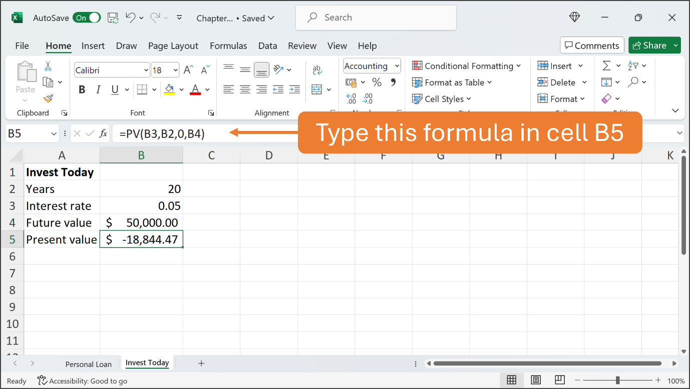
Type the contents in their respective cells. Use the default font and font size. You may format or adjust any column width if necessary. In cell B5, type the formula using the PV function, =PV(B3,B2,0,B4). Press Enter and you get the result.

Let’s look at each required component for the PV function.

The number of years is given as 20 in cell B2. The interest rate is written as 0.05, which translates to 5% in cell B3. The future value is given as $50,000 in cell B4. You can format the number in cell B4 to Accounting with the dollar symbol, $, and two decimal places.

The formula in cell B6 is written as =PV(B3,B2,0,B4) to get the amount that would be invested today. You can format the number in cell B4 to Accounting with the dollar symbol, $, and two decimal places. The result comes out in a negative value as it implies a cash outflow or in other words, the money you need to invest to get $50,000 in 20 years with an interest rate of 5%. You may get the result in red brackets indicating a negative value.

The first component, cell B3 is the interest rate, which is written as 0.05 or 5%. The second component, cell B2 is the number of periods, which is 20 years. The thirst component is the payment, and since there is no intervening payment, 0 is used in the formula. The fourth component, cell B4 is the future value, which is $50,0000.

As a result, Excel returns $ -18,844.47 in cell B5. It has a negative value as it means payments that should be made from you to the bank or cash outflow. You may get the value in brackets which also means a negative value.

That’s all for this Chapter.

You’re awesome!