Chapter 7: VLOOKUP Function

The VLOOKUP function accepts a value, then looks the value up in a vertical lookup table and returns a result. You can use the VLOOKUP function to search for exact matches or approximate matches.

In this chapter, you will learn two examples of the VLOOKUP function, one is to search for exact matches and the other is to search for the approximate matches.

The Figure below shows the first example of the VLOOKUP function which is to search for exact matches. This example allows you to type a fruit name in cell E1 and Excel will return the corresponding price in cell F1.

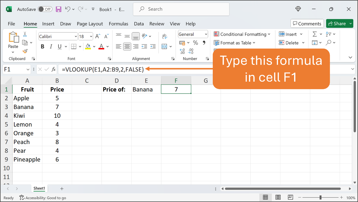
Type the contents in their respective cells. Use the default font and font size. You may bold and centre the content in each cell as shown in the Figure. Adjust any column width if necessary.

In cell F1, type the formula using the VLOOKUP function, =VLOOKUP(E1,A2:B9,2,FALSE). Press Enter and you get the result.

Using the VLOOKUP function, Excel looks for any matched value in the range of cells from cell A2 until cell A9 vertically based on the value in cell E1.

If the value in cell E1 is matched with any value in the range of cells from cell A2 until cell A9, Excel returns the corresponding value from column B. In this formula, column A is column number 1, and column B is column number 2. That is why, the range of cells should be from A2 until B9 or written as A2:B9 in the formula.

Column B or column number 2 is where the corresponding value is extracted. That is why, the column number in the formula is written as 2. The word FALSE in the formula instructs Excel only to search for an exact match from Column A or column number 1.

In this example, the value in cell E1 is Banana, where it matches the value in cell A3 in the range of cells. The corresponding value from column number 2 is 7. Thus, Excel returns 7 in cell F1.

If you replace the value in cell E1 with the other value, Excel will return the corresponding value from column number 2. For example, if you replace it with Orange, Excel will return 3 in cell F1. However, if you replace it with a value not in the range of cells such as Mango or just leave it blank, Excel will return #N/A in cell F1. This is how you use the VLOOKUP function to find an exact match from the range of cells.

Let’s save the workbook to Chapter7.xlsx or any file name you prefer.

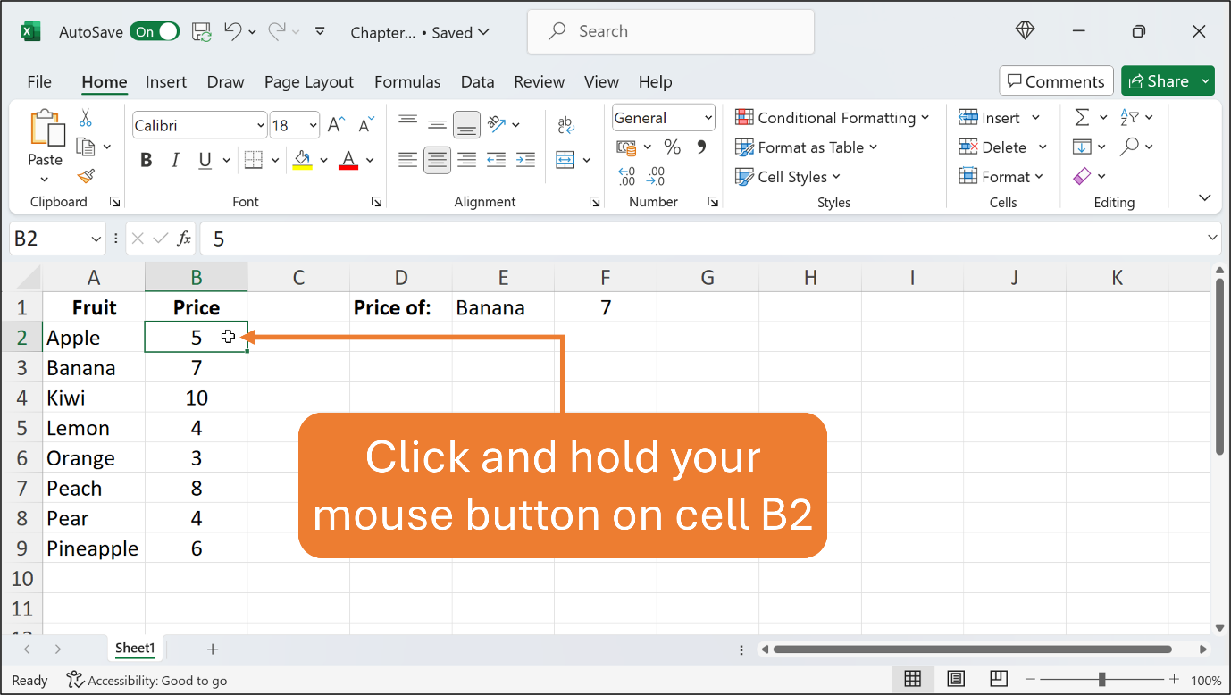
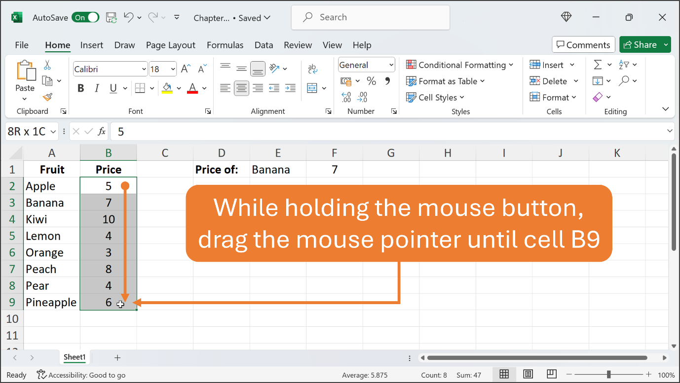
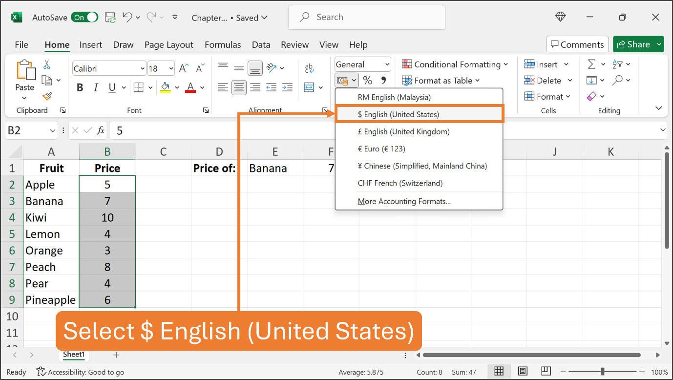
Go back to the worksheet and let’s format the numbers to the Accounting format with the dollar sign ($) symbol. The Accounting format is the most popular format for numbers, especially for creating financial statements and budgets.

See the Figures below to learn how to format the numbers to the Accounting format with the dollar sign ($) symbol.

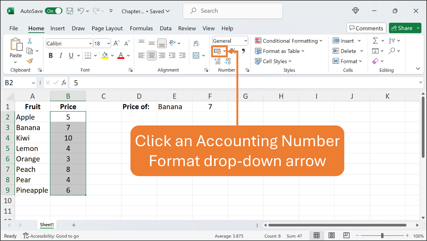
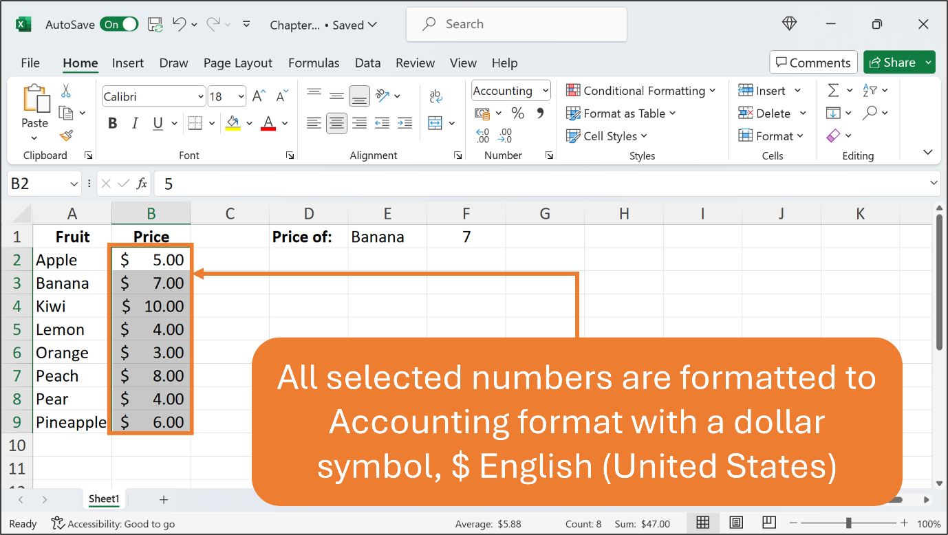
Now, you’re done with formatting the numbers to Accounting format with a dollar symbol, $ English (United States).

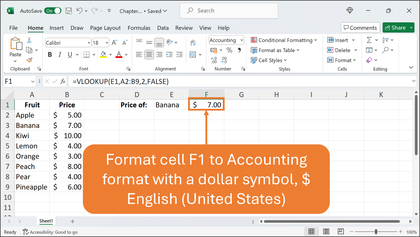
You can format cell F1 to Accounting format with the same steps as described in the above Figures.

You can change to another symbol depending on which currency you prefer.

The second example of the VLOOKUP function is to search for approximate matches.

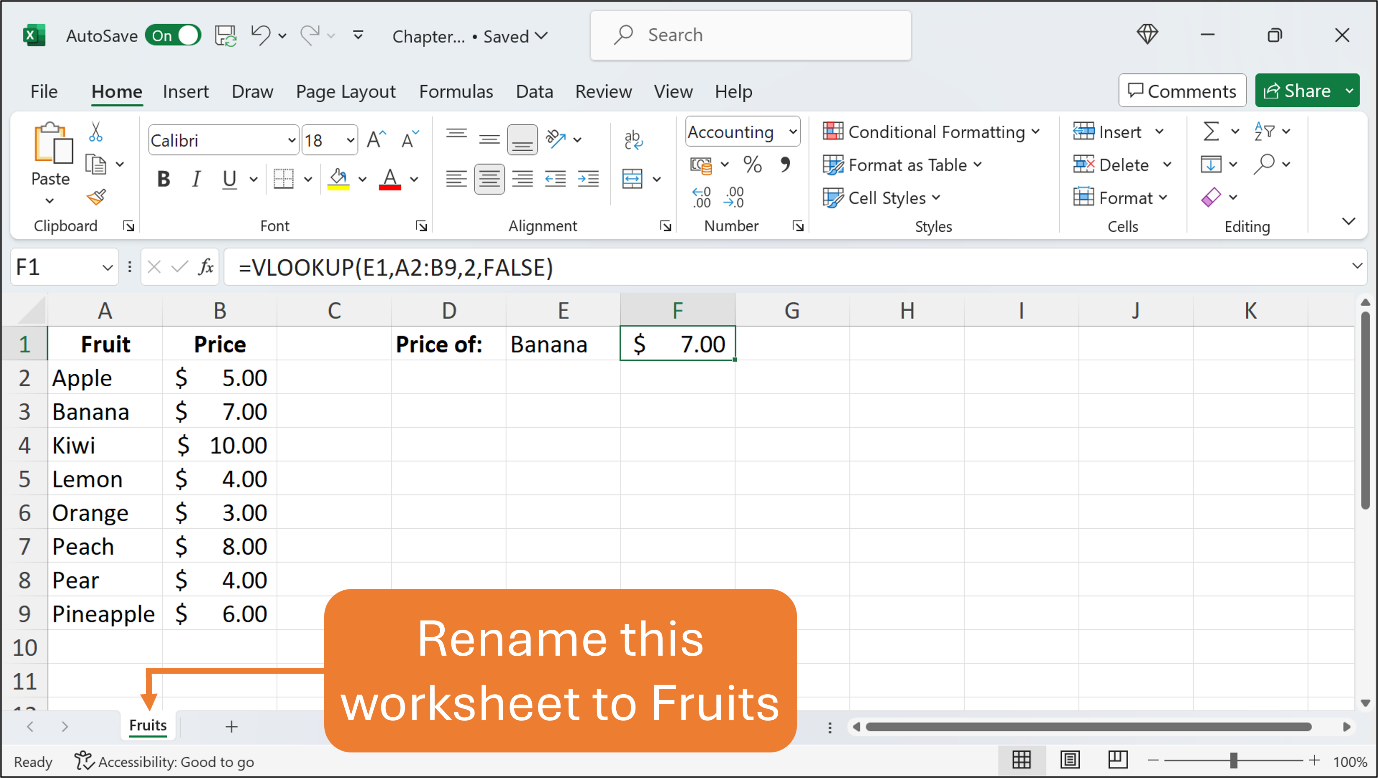
Before you proceed with the example, rename the current worksheet to Fruits. See the Figure below.

Then, insert the new worksheet and rename it to Sales and Commissions. See the Figure below.

The second example of the VLOOKUP function which is to search for approximate matches allows you to determine the commission rate in percentage (%) based on the sales made by each salesperson. See the Figure below. 

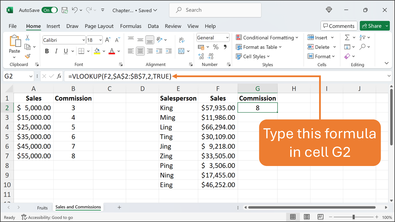
Type the contents in their respective cells. Use the default font and font size. You may bold and centre the content in each cell as shown in the Figure. Adjust any column width if necessary. You can format the numbers in Accounting format as described previously. In cell G2, type the formula using the VLOOKUP function, =VLOOKUP(F2,$A$2:$B$7,2,TRUE). Press Enter and you get the result.

Using the VLOOKUP function, Excel looks for any matched value in the range of cells from cell A2 until cell A7 vertically based on the value in cell F2. If the value in cell A2 is approximately matched with any value in the range of cells from cell A2 until cell A7, the Sales column, Excel returns the corresponding value from column B, the Commissions column. In the formula, column A is column number 1, and column B is column number 2. That is why, the range of cells should be from A2 until B7 or written as $A$2:$B$7 in the formula.

Note that this time, you should insert a dollar symbol, ($) in the cells to make them absolute references, as you are going to copy and paste the formula using the Fill handle later for the other cells in the same column.

Column B or column number 2 is where the corresponding value is extracted. That is why, the column number in the formula is written as 2. The word TRUE in the formula instructs Excel to search for approximate matches from Column A, the Sales column, or column number 1.

In this example, the value in cell F2 is $57,935.00, where it approximately matches or is greater than the value in cell A7, or the $55,000.00 breakpoint. Since the value or the lookup value in cell A7 is greater than the $55,000 breakpoint, and there is no breakpoint afterward, then Excel stays on that row. It then uses the column index number as written in the formula as number 2 to identify the column containing the value to return for the lookup value. The corresponding value from column number 2 is 8. Thus, Excel returns 8 in cell G2.

Do note that because Excel goes sequentially through the breakpoints. These breakpoints must be arranged from the lowest value to the highest value for ranges. If no exact match is found, Excel returns #N/A.

The Figure below shows when all Commissions have been calculated using the VLOOKUP function.

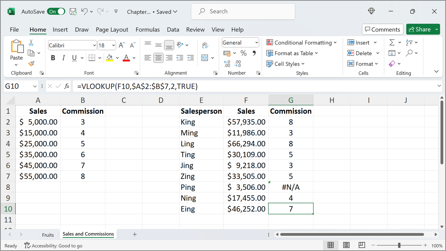
Do observe in the above Figure, that Excel returns #N/A in cell G8. This is because the value in cell G8 is no greater than the $5,000 breakpoint, thus no match and it is considered as no commission, or #N/A.

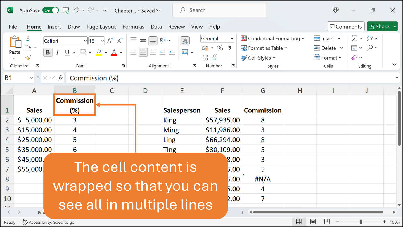
Now, let’s edit cells B1 and G1 to insert (%) at the end of the word Commission to make them more understandable for the worksheet presentation, and later wrap text both contents. See the Figures below.

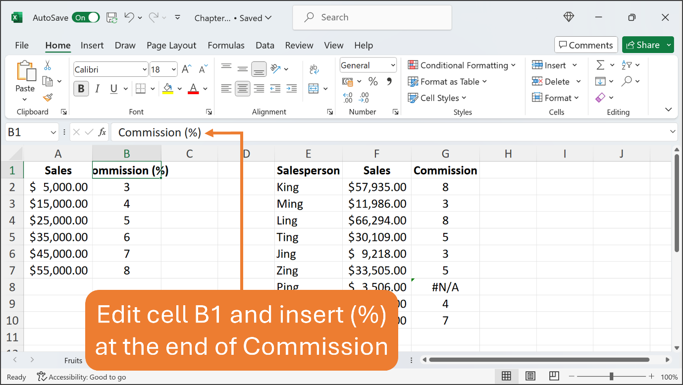
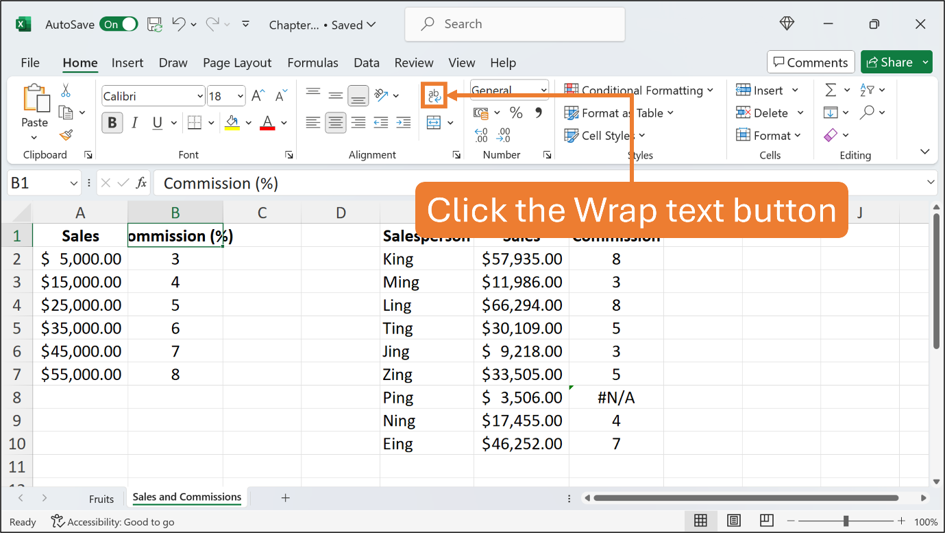
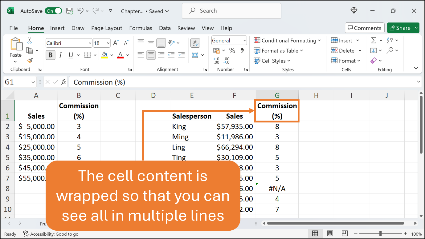
Follow the above Figures to edit cell G1 and to insert (%) at the end of the word Commission. Later, wrap the content in cell G1.

That’s all for this Chapter.

You’re awesome!