Chapter 2: Formula Basics

Knowing how to create formulas in Excel is mandatory. Formulas always start with an equal sign (=), which can be followed by a combination of numbers, cell references, mathematical operators, or functions. In this chapter, you will learn how to create basic Excel formulas using numbers and one of the following mathematical operators.

Let’s go!

Create a new blank workbook. Type the following contents in their respective cells as shown in the Figure below. Use the default font and size.

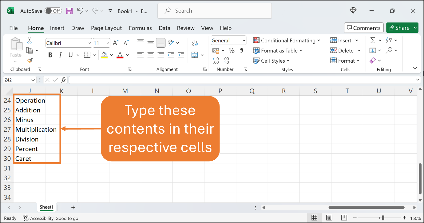
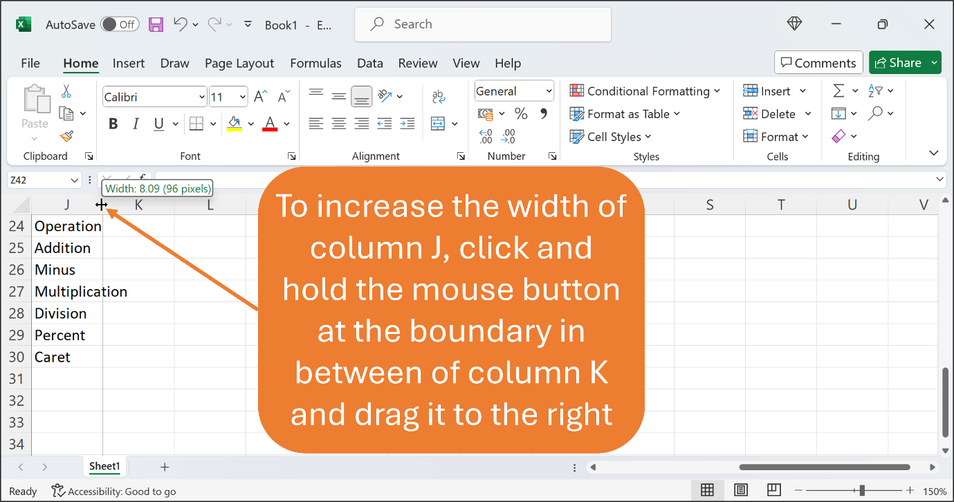
You will notice that one content in cell J27 overflows to the next cell in the next column. For your information, the default column size is 8.09 points or 96 pixels. Therefore, longer contents may flow into the next cell in the next column. To remedy this, we need to expand the width of column J. Bring your mouse pointer to the boundary in between column J and column K. Once the mouse pointer changes its shape to double-arrow, quickly hold your mouse button and drag it to the right to increase the width of column J.

See the Figure below.

When all contents in column J fit, then you can release the mouse button. Now you shall see the width of column J is longer or bigger than the widths of other columns.

See the Figure below.

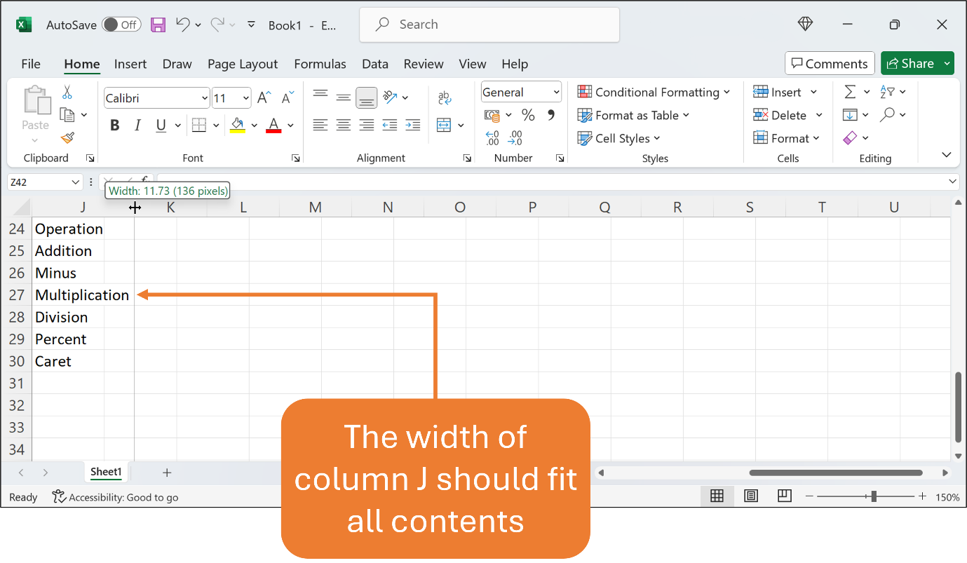
It is important to note that all contents are still in column J whether you expand the column width or not. However, for a better visual, it is recommended to expand the column width.

The other method to quickly expand the column width is to just double-click at the boundary, in this case, the boundary between column J and column K. Excel will adjust the width of column J automatically.

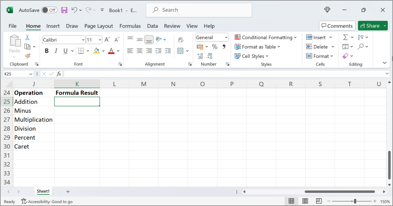
Now, type Formula Result in cell L24. Later, expand column L to fit the text.

Bold the contents in cell J24 and cell K24.

At this point, your worksheet should be as in the Figure below.

Now, save your workbook with your preferred name and in any location on your computer.

Let’s create the first formula.

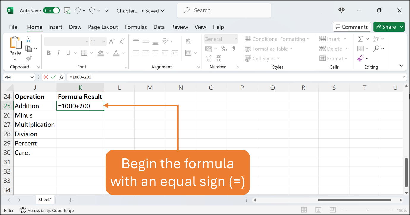
In this formula, we will use a plus symbol, (+) to add the values of two numbers, 1000 and 200.

In cell K25, create a formula to calculate 1000+200. Remember, an Excel formula should start with an equal sign (=). Type =1000+200 in cell K25, then press Enter. This is a very basic and straightforward formula just to show the use of a mathematical operator, a plus sign (+) for addition.

See the Figure below.

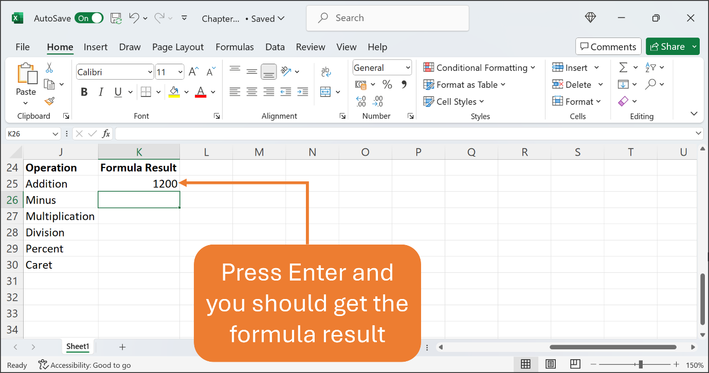
After typing the formula, press Enter to let Excel perform the calculation, 1000 + 200, and display the result in cell K25. As expected, Excel will display 1200 in cell K25. This is the formula result.

See the Figure below.

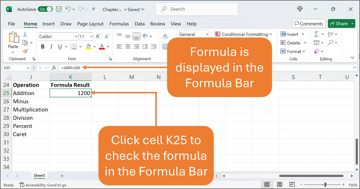
If you want to check or edit the formula, click cell K25 and the formula should be displayed in the Formula Bar. Double-click cell K25 to edit the formula if necessary.

See the Figure below.

At this stage, you should be able to understand the basic formula structure. The formula you have just created in cell K25 begins with an equal sign, (=) followed by the combination of two numbers and a plus sign, (+) for addition.

Now, by referring to the table that contains mathematical operators given at the beginning of this chapter, create a formula for each operation below.

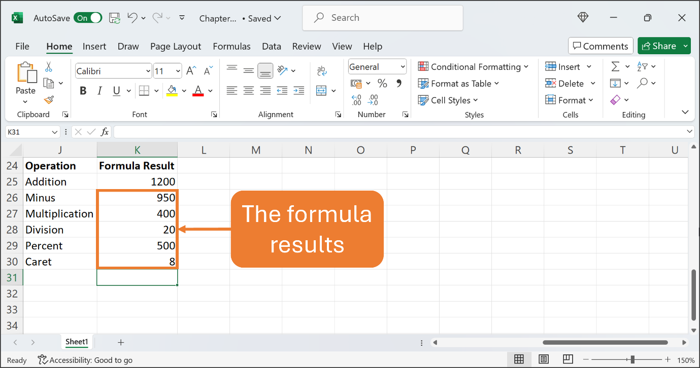
In cell K26, type =1000-50 as a formula to calculate 1000 – 50.

In cell K27, type =1000-50 as a formula to calculate 2 x 200.

In cell K28, type =1000/50 as a formula to calculate 1000 ÷ 50.

In cell K29, type 1000*50% as a formula to calculate 1000 x 50%.

In cell K30, type =2^3 as a formula to calculate 2^3.

The following figure shows the formula results.

That’s all for this Chapter.

You’re awesome!