Chapter 6: IF Function

This is one of the most popular functions in Excel where you can make logical comparisons between a value and what you expect. In other words, you can have two results from the IF function. The first result is if your comparison is True, and the second is if your comparison is False. It should be either the first or second result depending on True or False.

Let’s learn the IF function.

The Figure below shows an example using the IF function.

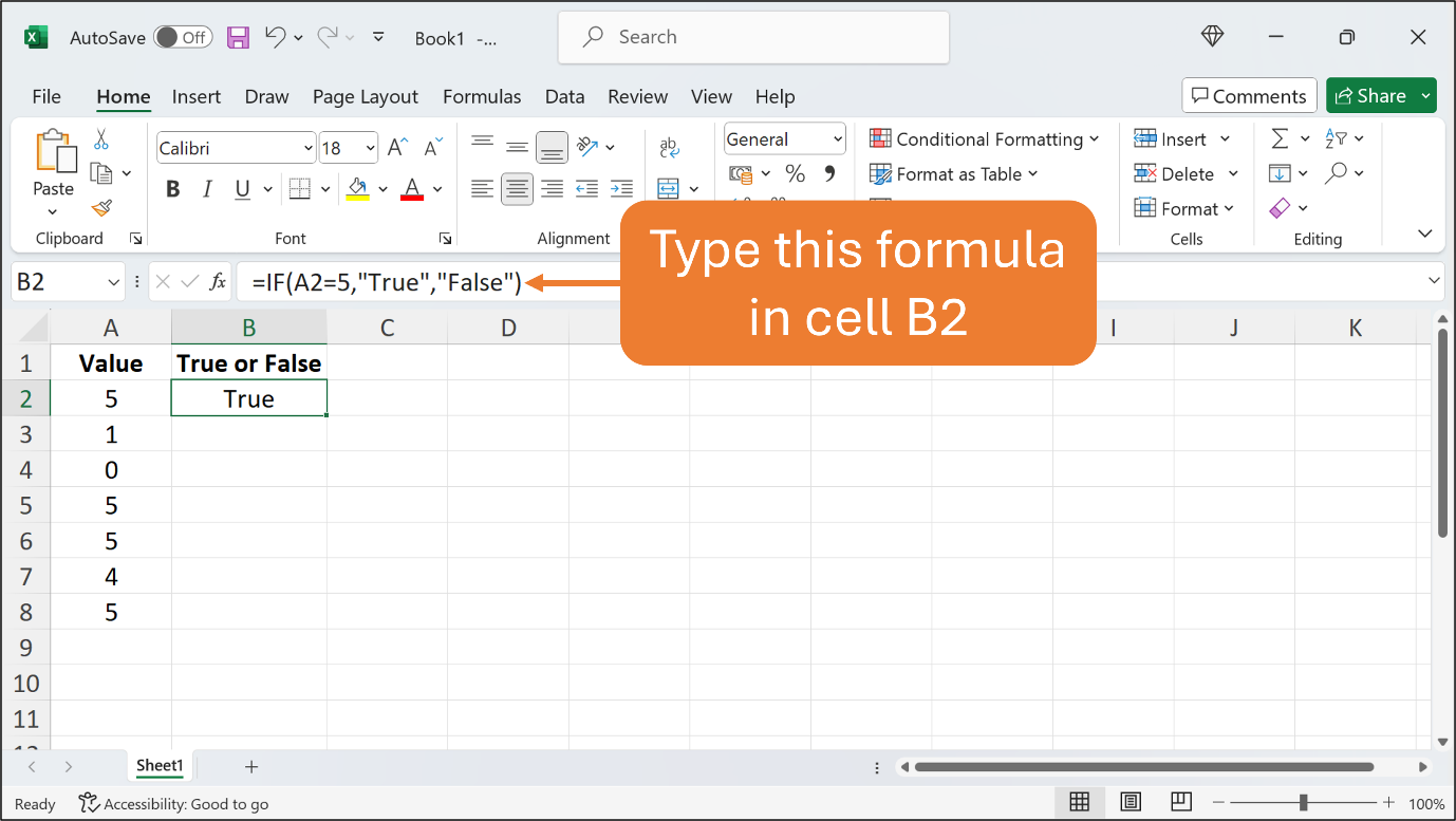
Type the contents in their respective cells. Use the default font and font size. You may bold and centre the content in each cell as shown in the Figure. Adjust any column width if necessary.

In cell B2, type the formula using the IF function, =IF(A2=5,“True”,“False”). Press Enter and you get the result. Excel returns True as the result in cell B2 as the logical comparison A2=5 is correct.

The logical comparison is whether A2=5 and since cell A2 contains 5, the logical comparison is True. Excel therefore returns True in cell B2, otherwise False if cell A2 contains other value other than 5.

Now, copy the formula in cell B2 and paste it to the remaining cells in the same column until cell B8 using the Fill Handle.

The Figure below shows all cells in column B have been filled with the formulas using the IF function.

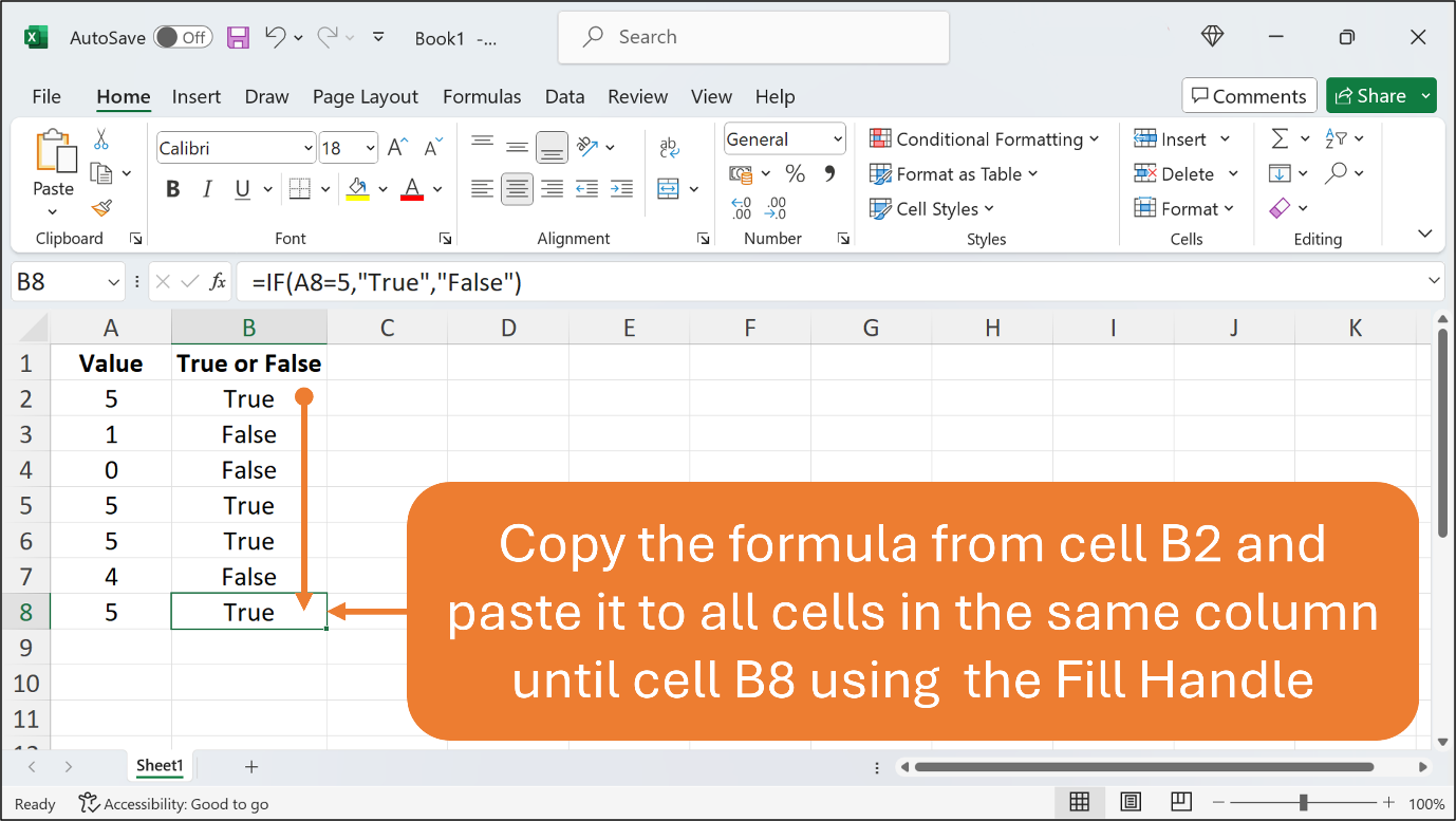
You can observe from the above Figure that cells B5, B6, and B8 have True results since the values are equal to 5 respectively.

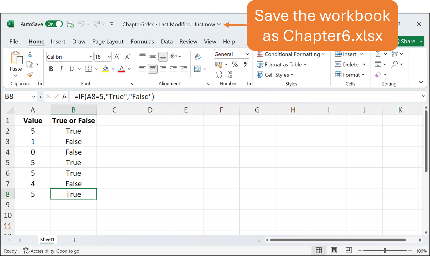
You can save this workbook using any file name or Chapter6.xlsx as shown in the Figure below.

Let’s learn the second example of the IF function.

You are going to create another worksheet for the second example of the IF function in the same workbook.

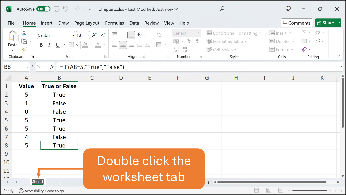
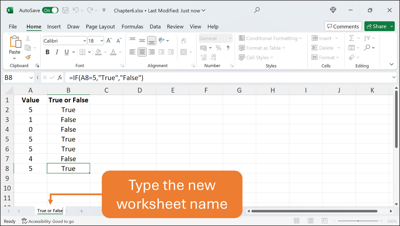
Before you proceed, rename the current worksheet name from Sheet1 to True or False. Double-click the worksheet tab and straight away type the new worksheet name.

See the Figures below.

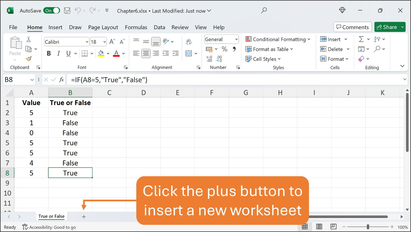
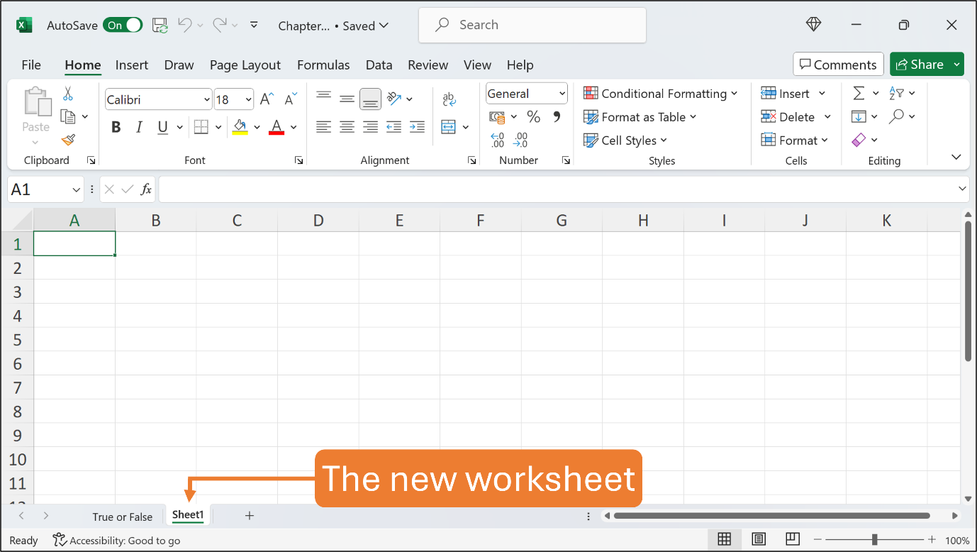
Now, insert a new worksheet. Click the plus (+) button on the right of the worksheet tab and a new worksheet is inserted immediately and you can type the new worksheet name. See the Figures below.

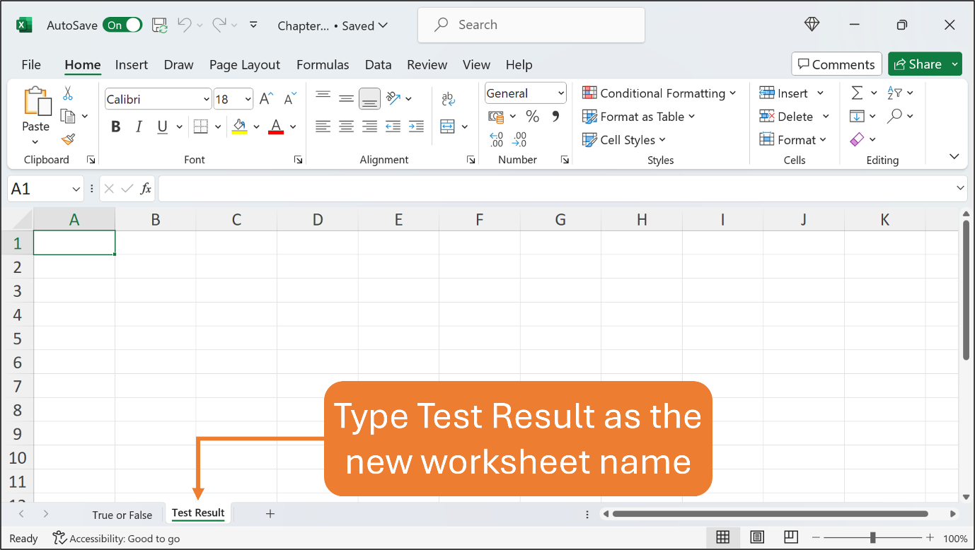
Rename the new worksheet as Test Result. See the Figure below.

The second example of the IF function is illustrated in the Figure below.

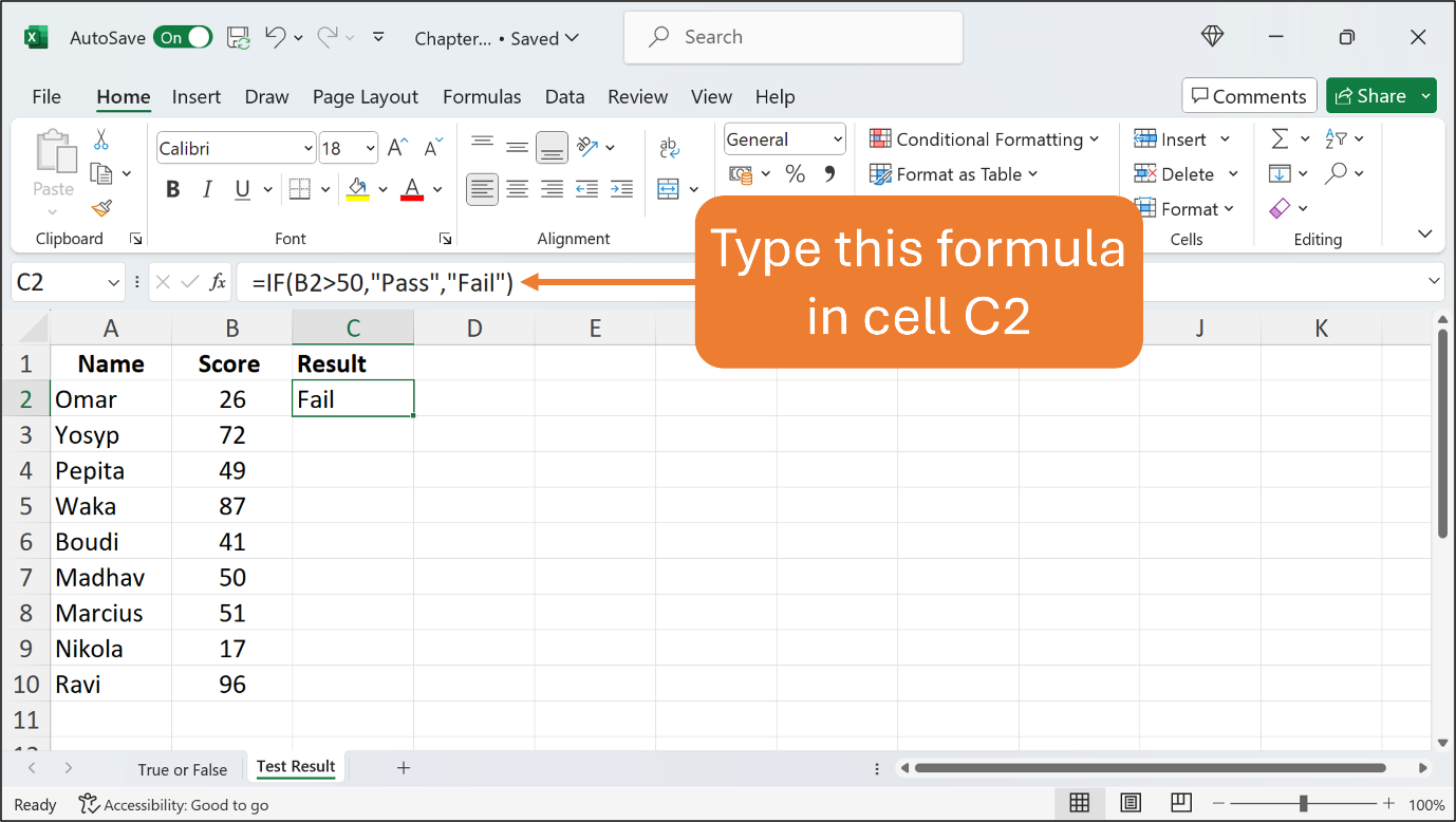
Type the contents in their respective cells. Use the default font and font size. You may bold and centre the content in each cell as shown in the Figure. Adjust any column width if necessary.

In cell C2, type the formula using the IF function, =IF(B2>50,“Pass”,“Fail”). Press Enter and you get the result as Fail as displayed in cell C2. The formula instructs Excel to determine whether the logical comparison of the value in cell B2 is greater than 50 (B2>50), but since it is 26 which is less than 50, Excel returns Fail in cell C2. Unlike the first example, False is replaced by Fail as it is written in the formula. In other words, Excel returns a False statement according to the IF formula.

The formula can be read, if a value in cell B2 is greater than 50, then Pass will be displayed (True), or if a value in cell B2 is less than 50, then Fail will be displayed (False).

Now, copy the formula in cell C2 and paste it to the remaining cells in the same column until cell C10 using the Fill Handle.

The Figure below shows all cells in column C have been filled with the formulas using the IF function.

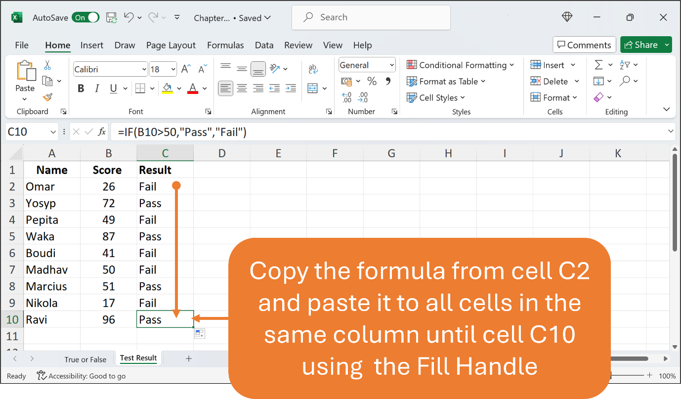
You can observe from the above Figure that cells C3, C5, C8, and C10 have Pass results since the scores are greater than 50 (>50) respectively. Cells C4, C6, C7, and C7 show the Fail results as the scores are less than 50.

In using the IF function, you can use the following logical operators to make the comparison in the logical test.

See below.

The IF function lets you make informed decisions based on the data on the worksheet.

That’s all for this Chapter.

You’re awesome!